1 Modeling

1.1 Overview

The architecture is built using MATLAB/Simulink and Simscape, following a Multi Domain Model Design approach. The system is explicitly divided into two referenced models to separate the discrete software logic from the continuous physical plant:

• control_<axis>: The discrete-time control algorithm (firmware replica).
• machine_<axis>: The continuous-time physical model (Simscape Multibody/Foundation).

The repository is available here.

1.2 Top-Level Integration

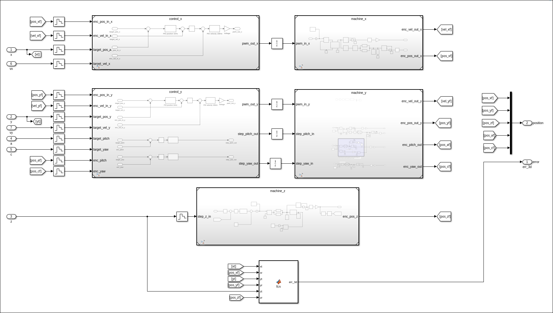
The top-level model connects the control logic and the physical plant. Since the controller operates in the discrete-time domain (simulating an STM32 microcontroller) and the physical plant operates in the continuous-time domain, appropriate interface blocks are utilized:

• Zero-Order Hold (ZOH): Applied to the continuous feedback signals (position and velocity) entering the controller. This mimics the finite sampling rate of the microcontroller’s timers and real-time.
• Unit Delay (\(z^{-1}\)): Placed between the controller’s PWM output and the plant’s input. This breaks the algebraic loop, accurately simulating the computational delay (e.g., 100 \(\mu s\)) between reading the encoders and updating the motor driver.

Overall

1.3 X: Extruder Axis

1.3.1 Control sub-Model

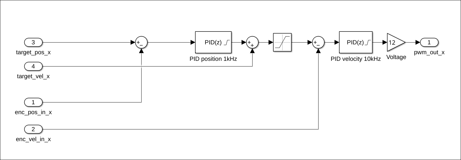
The control logic features a discrete cascade PID architecture with feedforward compensation, matching the physical C firmware structure:

• Outer Position Loop (1 kHz): Computes the positional error. The positional feedback is quantized to simulate the finite resolution of the RLS linear encoder. The output of this PID(z) is a baseline velocity command.
• Velocity Feedforward: The target feedrate is directly summed with the output of the position PID. This acts as a primary driving signal, allowing the position PID to operate purely as a low-effort error corrector (usually purely Proportional), avoiding heavy oscillations.
• Inner Velocity Loop (10 kHz): Compares the feedforward-adjusted target velocity against the quantized feedback from the AS5048A rotary encoder. This highly responsive PID(z) outputs a normalized duty cycle, which is then amplified by the system voltage (e.g., 12V) to command the physical motor.

control_x

1.3.2 Physical Plant sub-Model

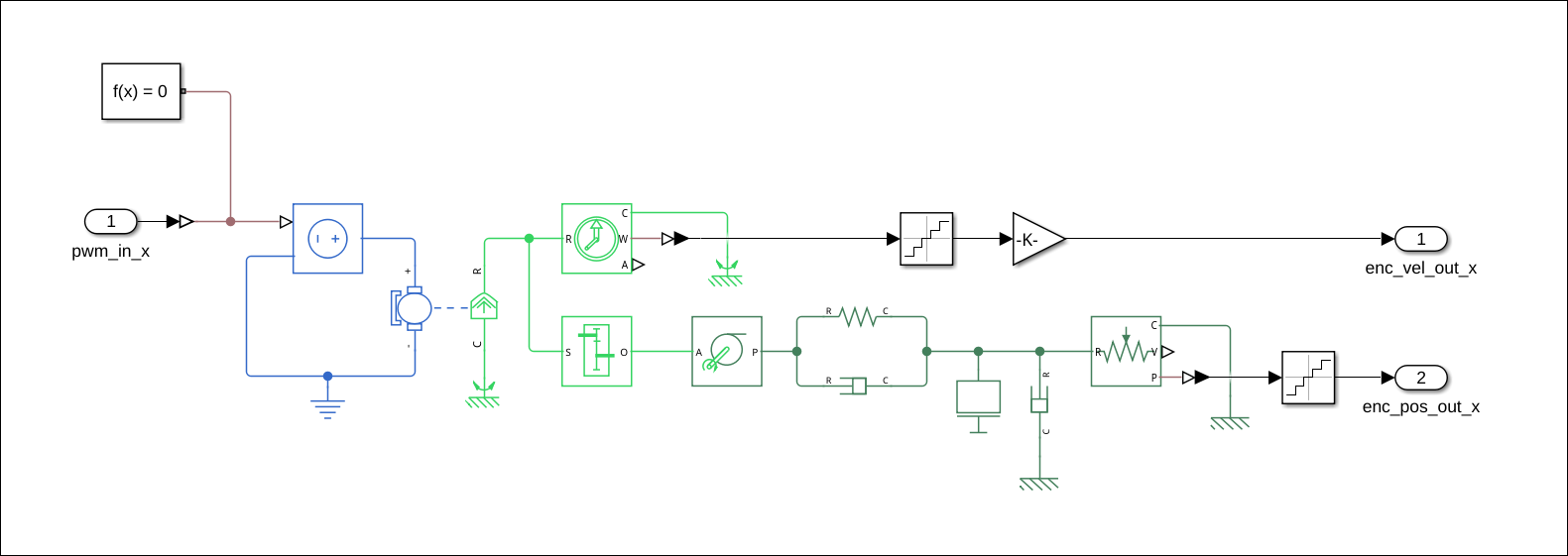
The plant is modeled using the Simscape Foundation Library, employing a physical network approach rather than purely signal-based mathematical blocks. This ensures accurate bidirectional power flow and energy conservation across different physical domains (Electrical, Rotational, and Translational).

model_x

1.3.2.1 Domain Boundary and Electrical Circuit

The flow begins with the pwm_in signal coming from the discrete controller. Since this is a standard Simulink mathematical signal, it first passes through a Simulink-PS Converter to enter the physical domain. This signal drives a Controlled Voltage Source, establishing the electrical circuit against an Electrical Reference (ground). The generated voltage powers the DC Motor block, which is parameterized with real-world electrical constraints (armature resistance, inductance, and back-EMF) and mechanical rotor inertia.

1.3.2.2 Rotational Mechanics and Sensing

The DC Motor converts electrical power into mechanical rotational power. Its casing is anchored to a Mechanical Rotational Reference, while the shaft output connects to a primary rotational node. From this node, the network branches out to handle both sensing and power transmission:

• Velocity Feedback: An Ideal Rotational Motion Sensor taps into the shaft to measure the angular velocity. The physical measurement is sent through a PS-Simulink Converter to become the enc_vel_out signal, feeding the inner PID loop.
• Torque Monitoring: An Ideal Torque Sensor is placed in series with a secondary ground to measure the effort generated by the motor, outputting the data to a Scope (Torque monitor) for tuning and diagnostic purposes.

1.3.2.3 Transmission and Flexible Coupling

The main rotational power flows into a Wheel and Axle block, which acts as the drive pulley, converting the angular motion into linear displacement. Crucially, the timing belt connecting the pulley to the carriage is not modeled as a perfectly rigid link. The linear output passes through a parallel combination of a Translational Spring and a Translational Damper. This setup accurately captures the mechanical compliance, structural resonance, and internal high-frequency energy dissipation (“ringing”) inherent in belt-driven systems.

1.3.2.4 Linear Dynamics and Position Feedback

Following the flexible transmission, the linear force pulls the Mass block, representing the physical weight and inertia of the extruder carriage. To simulate the viscous friction of the linear recirculating ball bearing guides, a secondary Translational Damper is connected between the mass and the Mechanical Translational Reference (the physical ground of the machine). Finally, an Ideal Translational Motion Sensor is connected to the carriage mass. It reads the absolute physical position without drawing energy from the system, passing the measurement through a PS-Simulink Converter to generate the enc_pos_out signal for the outer positional PID loop.

1.4 Y: Printing Plate Axis

1.4.1 Control sub-Model

The control logic for the Y-axis utilizes the exact same discrete cascade PID architecture with velocity feedforward as the X-axis. By leveraging Simulink’s Model Reference arguments, the identical control model is instantiated with a specific set of tuning parameters (\(K_p\), \(K_i\), \(K_d\), and saturation limits) tailored to the heavier load and different resonant frequencies of the Y-axis.

1.4.1.1 Rotational Axis Control

As regards the additional A and C axis (respectively global pitch and plate-local yaw), control law is simplified: at first, stepper motors are used, and second, just the rotating encoder AS5048A is embedded on the rotating shaft. Thanks to that, it is possible to implement a fast PID (10kHz frequency) by means of just Proportional gain. Derivative and Integral term are null for the C axis, while the A axis uses a small derivative term in order to smooth the kickback to the Y-axis carriage.

1.4.2 Physical Plant sub-Model

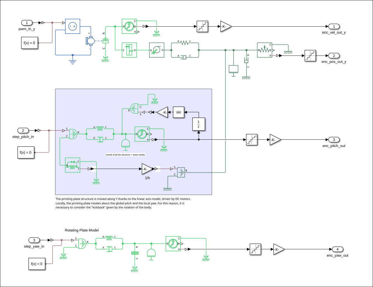
The core physical network (machine_y), encompassing the electro-mechanical conversion (DC Motor) and the flexible transmission (belt elasticity and damping), remains structurally identical to the extruder axis. However, the load characteristics are significantly more complex due to the multi-axis mechanical linkages.

1.4.3 Coupled Dynamics: The Pendulum Effect and Tangential Kickback

The primary distinction in the Y-axis physical model lies in the Mass block and its external inputs. The Y-axis carriage supports the entire printing plate and the rotating cradle (Pitch axis), introducing severe parasitic dynamics that the control loops must mathematically reject.

• The Pendulum Effect (Gravity Bias): Unlike a perfectly balanced rotational load, the Center of Gravity (CG) of the Pitch cradle is mechanically offset from its axis of rotation. Consequently, gravity continuously exerts a variable torque on the Pitch axis. This is calculated using the exact physical formula: \(\tau_{g} = m \cdot g \cdot d_{CG} \cdot \sin(\theta_{pitch})\), where \(m\) is the mass of the cradle, \(g\) is the gravitational acceleration (\(9.81 m/s^2\)), and \(d_{CG}\) is the offset distance of the center of gravity. This introduces a non-linear pendulum effect. In the model, this is simulated using a trigonometric function block fed by the instantaneous pitch angle, which dynamically calculates and injects this gravitational load into the rotational physical network.

• Tangential Kickback (Reaction Force): Furthermore, the Pitch and Y axes are strictly coupled through Newton’s Third Law. Whenever the Pitch stepper motor violently accelerates the heavy cradle, an equal and opposite reaction torque is exerted on the motor’s stator, which is rigidly mounted to the Y-axis carriage. Because of the geometric lever arm (\(h\)), this reaction torque translates into a tangential linear force (kickback) acting directly along the Y-axis guides.

To accurately capture this multi-domain coupling without resorting to computationally heavy 3D Multibody DAE solvers, an active signal routing technique is implemented in Simscape: an Ideal Torque Sensor measures the rotational effort of the cradle, scales it by the inverse of the center of percussion distance (\(1/h\)), and injects it back into the Y-axis translational node via an Ideal Force Source. This ensures the Digital Twin faithfully represents the sudden linear disturbances the Y-axis cascade controller must actively counteract during simultaneous 5-axis movements.

model_y

1.4.3.1 Yaw-Rotating Printing Plate

On the other hand, the printing plate also rotates on its own Z-axis, defining the 5th global printing axis. The rotational model of the Yaw plate is structurally similar to the Pitch axis, differentiated primarily by its specific inertial mass and viscous damping values. Since its axis of rotation is orthogonal to the Y-axis translation, its dynamic coupling is less invasive compared to the Pitch kickback.

1.5 Z: Vertical Positioning Axis

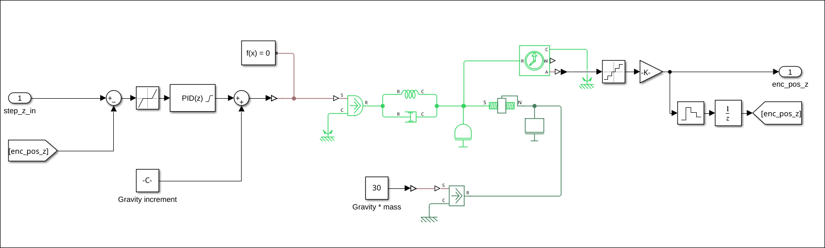
Unlike the X and Y axes, which utilize closed-loop DC motors for high-speed dynamic movements, the Z-axis is responsible for precise, low-speed vertical positioning. As poisitioning axis, a stepper motor is exploited. The input step_z_in is a standardized signal representing the desired discrete steps.

The Z-axis physical model translates discrete step commands into physical vertical motion, factoring in the unique properties of a lead screw transmission.

model_z

1.5.1 Stepper Translation

The input step signal is passed through an Ideal Torque Source (via a Gain block to convert steps to velocity). This enforces a strict kinematic translation profile, simulating the rigid holding torque and discrete stepping nature of the motor without modeling the complex electromagnetics of the stepper coils. This is just a modeling escamotage.

1.5.2 Transmission and Leadscrew Dynamics

The core element of the Z-axis is the Translational Spring and Translational Damper assembly, acting as a flexible coupling between the ideal step source and the physical carriage. This captures the mechanical compliance (backlash and axial deformation) of the lead screw nut when subjected to varying loads. The rotational-to-linear conversion of the lead screw is abstracted into the step-to-translation gain.

1.5.3 Mass and Gravity Bias

The entire weight of the gantry acts continuously on the Z-axis. This is modeled using an Ideal Force Source injecting a constant downward force equal to Gravity * mass (\(9.81 \cdot 3\) kg). The carriage itself is represented by a Mass block, and a Translational Damper simulates the friction of the vertical rails. This setup ensures the system accurately models the asymmetrical effort required to lift the gantry versus lowering it, and the resting deflection of the flexible transmission.

1.6 Model validation

Before deploying advanced model-based control strategies, it is strictly necessary to validate the fidelity of the Simscape physical network. The objective of this phase is to ensure that the FMU (Digital Twin) accurately replicates the dynamic behavior of the real 5-axis kinematics when subjected to the same stimuli.

To achieve this, an open-loop and closed-loop validation procedure was conducted. The physical machine and the FMU were fed identical trajectory profiles (position and velocity setpoints), and their respective outputs were logged and compared.

1.6.1 Trajectory Tracking Comparison

A standard testing routine—comprising sharp accelerations, cruising speeds, and direction reversals—was executed on the physical hardware. The identical control signals were passed to the FMU running in parallel.

Position and Velocity Tracking Comparison

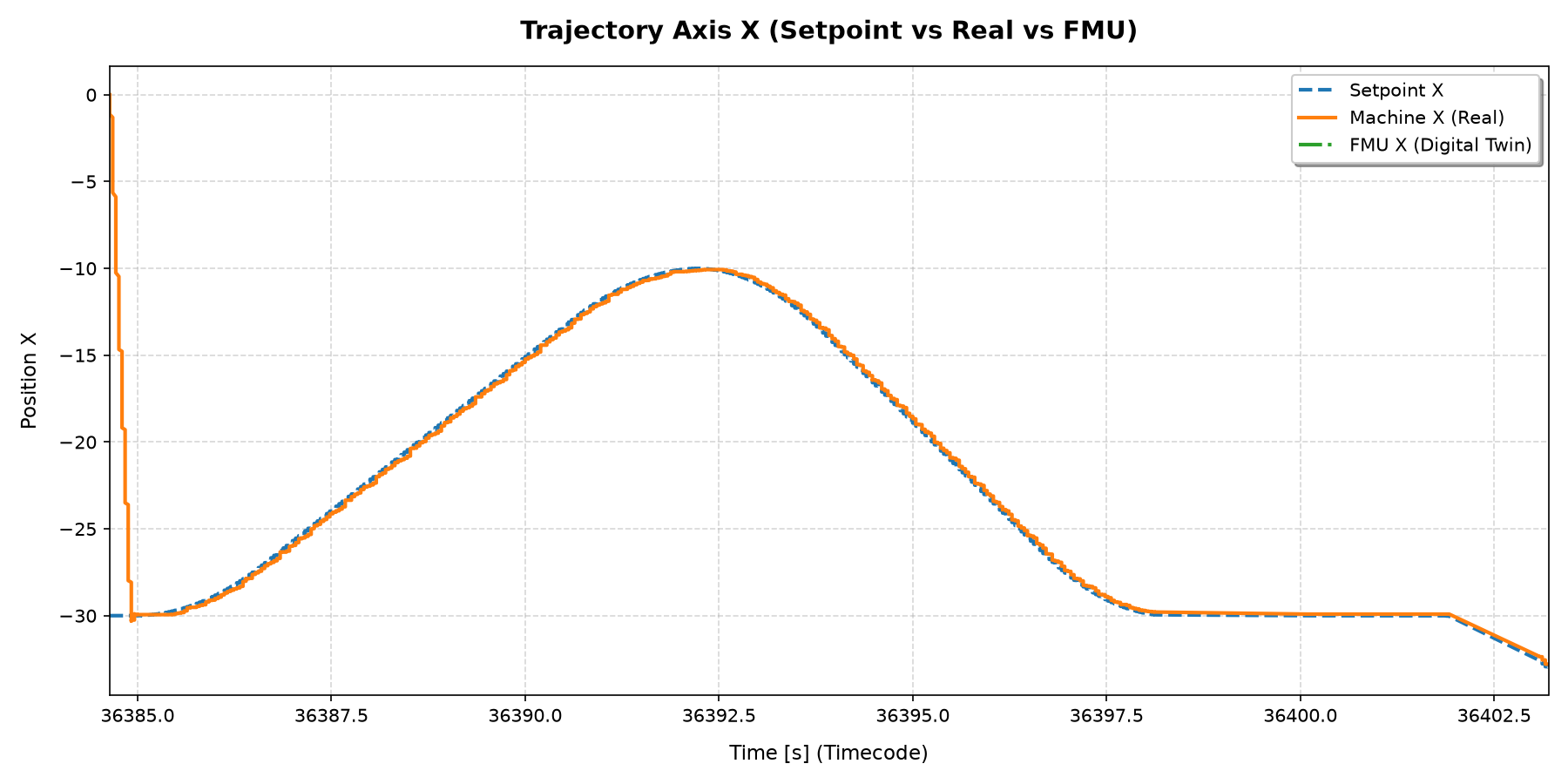
As observed in the plot, the baseline 1D multidomain model successfully captures the dominant dynamics of the system. The mechanical compliance (belt stretching), the inertial resistance, and the Pitch-to-Y kickback coupling are faithfully simulated, maintaining the simulated trajectory within an acceptable error margin from the physical ground truth.

1.6.2 Residual Error and the Need for Adaptation

The residual tracking errors expose a fundamental limitation of static modeling: parameter variability.

While geometric constants (like the center of gravity distance \(d_{CG}\) or motor torque constants \(K_t\)) remain fixed, other crucial parameters change continuously during operation:

1. Dynamic Payload: The equivalent mass of the Y-axis and the rotational inertia of the Pitch and Yaw axes increase steadily as plastic material is extruded onto the printing plate.
2. Thermal Variations: The viscous friction coefficients (\(B\)) of the linear guides and the belt damping factors vary as the mechanical components heat up during long printing sessions.

Relying on a statically calibrated FMU would lead to a progressive deterioration of the feedforward compensation and model-predictive features. To bridge this gap and achieve perfect alignment between the Digital Twin and the physical machine, the static parameters must be dynamically updated. This requirement naturally introduces the implementation of an Online Parameter Identification strategy.